Using PMLB Python interface
message("Current working directory: ", getwd())
message("Contents of working directory: ", paste(dir(getwd()), collapse = ", "))
Install
Most users should install PMLB from the Python Package Index (PyPI)
using pip:
For access to new features or datasets that are not yet merged into an official release, you can instead install from the GitHub sources:
Usage
from pmlb import fetch_data

# Returns a pandas DataFrame
mushroom = fetch_data('mushroom')
mushroom.describe().transpose()
## count mean std min 25% 50% 75% max
## cap-shape 8124.0 2.491876 0.901287 0.0 2.0 2.0 3.0 5.0
## cap-surface 8124.0 1.742984 1.179629 0.0 0.0 2.0 3.0 3.0
## cap-color 8124.0 4.323486 3.444391 0.0 0.0 3.0 8.0 9.0
## bruises? 8124.0 0.584441 0.492848 0.0 0.0 1.0 1.0 1.0
## odor 8124.0 4.788282 1.983678 0.0 4.0 6.0 6.0 8.0
## gill-attachment 8124.0 0.974151 0.158695 0.0 1.0 1.0 1.0 1.0
## gill-spacing 8124.0 0.161497 0.368011 0.0 0.0 0.0 0.0 1.0
## gill-size 8124.0 0.309207 0.462195 0.0 0.0 0.0 1.0 1.0
## gill-color 8124.0 4.729444 3.342402 0.0 2.0 4.0 7.0 11.0
## stalk-shape 8124.0 0.567208 0.495493 0.0 0.0 1.0 1.0 1.0
## stalk-root 8124.0 1.109798 1.061106 0.0 0.0 1.0 1.0 4.0
## stalk-surface-above-ring 8124.0 2.498277 0.814658 0.0 2.0 3.0 3.0 3.0
## stalk-surface-below-ring 8124.0 2.424914 0.870347 0.0 2.0 3.0 3.0 3.0
## stalk-color-above-ring 8124.0 5.446578 2.143900 0.0 5.0 7.0 7.0 8.0
## stalk-color-below-ring 8124.0 5.393402 2.194604 0.0 5.0 7.0 7.0 8.0
## veil-type 8124.0 0.000000 0.000000 0.0 0.0 0.0 0.0 0.0
## veil-color 8124.0 1.965534 0.242669 0.0 2.0 2.0 2.0 3.0
## ring-number 8124.0 1.069424 0.271064 0.0 1.0 1.0 1.0 2.0
## ring-type 8124.0 2.291974 1.801672 0.0 0.0 2.0 4.0 4.0
## spore-print-color 8124.0 3.062038 2.825308 0.0 1.0 3.0 7.0 8.0
## population 8124.0 3.644018 1.252082 0.0 3.0 4.0 4.0 5.0
## habitat 8124.0 3.221073 2.530692 0.0 0.0 3.0 6.0 6.0
## target 8124.0 0.482029 0.499708 0.0 0.0 0.0 1.0 1.0## (8124, 23)The fetch_data function has two additional
parameters:
return_X_y(True/False): Whether to return the data in scikit-learn format, with the features and labels stored in separate NumPy arrays.local_cache_dir(string): The directory on your local machine to store the data files so you don’t have to fetch them over the web again. By default, the wrapper does not use a local cache directory.
For example:
from pmlb import fetch_data

# Returns NumPy arrays
mush_X, mush_y = fetch_data('mushroom', return_X_y=True, local_cache_dir='../datasets')
mush_X.shape
## (8124, 22)## (8124,)You can also list the available datasets as follows:
import random
from pmlb import dataset_names, classification_dataset_names, regression_dataset_names

rand_datasets = random.choices(dataset_names, k=7)
print('7 arbitrary datasets from PMLB:\n', '\n '.join(rand_datasets))
## 7 arbitrary datasets from PMLB:
## feynman_II_3_24
## 608_fri_c3_1000_10
## tic_tac_toe
## analcatdata_cyyoung9302
## 1096_FacultySalaries
## first_principles_rydberg
## 626_fri_c2_500_50print(
f'PMLB has {len(classification_dataset_names)} classification datasets '
f'and {len(regression_dataset_names)} regression datasets.'
)## PMLB has 179 classification datasets and 271 regression datasets.Example benchmarking
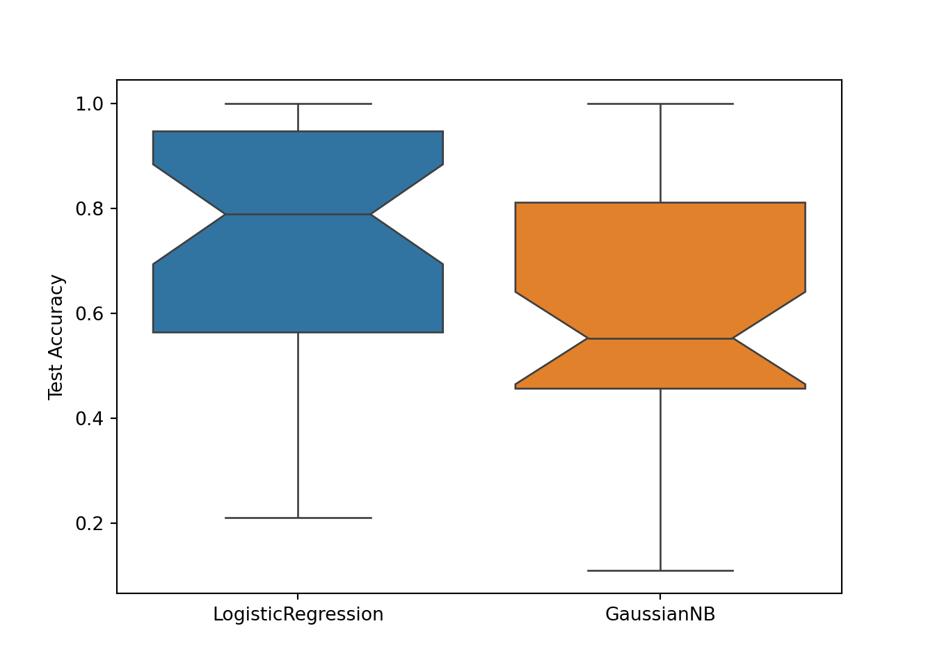
PMLB is designed to make it easy to benchmark machine learning algorithms against each other. Below is a Python code snippet showing the a sample comparison of two classification algorithms on the first 40 PMLB datasets.
from sklearn.linear_model import LogisticRegression
from sklearn.naive_bayes import GaussianNB
from sklearn.model_selection import train_test_split

import matplotlib.pyplot as plt
import seaborn as sb

from pmlb import fetch_data, classification_dataset_names

logit_test_scores = []
gnb_test_scores = []

classification_dataset_names = [
    name for name in classification_dataset_names if not name.startswith("_deprecated_")
]

for classification_dataset in classification_dataset_names[:40]:
    # Read in the datasets and split them into training/testing
    X, y = fetch_data(classification_dataset, return_X_y=True)
    train_X, test_X, train_y, test_y = train_test_split(X, y)

    # Fit two sklearn algorithms:
    # Logistic regression and Gaussian Naive Bayes
    logit = LogisticRegression()
    gnb = GaussianNB()
    logit.fit(train_X, train_y)
    gnb.fit(train_X, train_y)

    # Log the performance score on the test set
    logit_test_scores.append(logit.score(test_X, test_y))
gnb_test_scores.append(gnb.score(test_X, test_y))GaussianNB()In a Jupyter environment, please rerun this cell to show the HTML representation or trust the notebook.
On GitHub, the HTML representation is unable to render, please try loading this page with nbviewer.org.
GaussianNB()
# Visualize the result:
sb.boxplot(data=[logit_test_scores, gnb_test_scores], notch=True)
plt.xticks([0, 1], ['LogisticRegression', 'GaussianNB'])
## ([<matplotlib.axis.XTick object at 0x7fa188d79850>, <matplotlib.axis.XTick object at 0x7fa189713090>], [Text(0, 0, 'LogisticRegression'), Text(1, 0, 'GaussianNB')])